Excel Cell Search & Calc

Thanks to my buddy Ron for this challenge...

The Excel Formula below is handy when you want to search for a specific value contained within an adjacent cell and then do a calculation of time that rounds up to the nearest quarter hour.  This formula includes error trapping if the searchable cell contains a null value.


=IFERROR(CEILING(IF(OR(ISNUMBER(SEARCH("*R*",H2)),ISNUMBER(SEARCH("*A*",H2))),AD2,IF(ISNUMBER(SEARCH("*C*",H2)),AD2*DataRef!$B$1,IF(ISNUMBER(SEARCH("*I*",H2)),AD2*DataRef!$B$2,""))),0.25),"")

Excel "In Between"

This Excel example will show you how to determine if a cell value is "In Between" a pre-established range. Please see the details below for setup steps and a visual example...

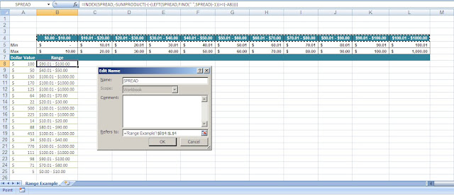
Example Assumptions:

• The spreadsheet has been named: Range Example
• This cell value that you wish to calculate is: A8
• The 'in between' values to check against are placed in cells: B4:L4

Setup Steps:

1. Create your "in between" values somewhere on the spreadsheet (Cells B4:L4 are used in this example)
2. Create a "Named Range". In this example, the Named Range has been called: "SPREAD".
3. In the "Refers to:" field for "SPREAD", enter the following reference: ='Range Example'!$B$4:$L$4
4. Click 'OK' to save the Named Range.
5. Enter the formula below into a cell that's (preferably) adjacent to the cell that you wish to find the range for:

=INDEX(SPREAD,-SUMPRODUCT(-(-(LEFT(SPREAD,FIND(" ",SPREAD)-1))>=(-A8))))

The formula above uses the "SPREAD" Named Range, which you defined earlier, to determine if the referenced cell is 'in between' the pre-established range.

For a visual representation of how to set this up, please see the screen shot below...

Dynamic Range Assignment

Dynamic Referencing for Excel Pivot Table(s) and / or Graph(s)

BC, this one's for you... :-)

Situation: You have an Excel solution that auto generates Graphs and / or Charts based on a specific set of data that changes over time. Instead of manually re-selecting a new Data Source for your Pivot Table(s) and / or Graph(s) each time your Raw Data changes (i.e. appending Q2 data to Q1, etc.), check out the information below for a dynamic solution...

• Excel Sheet Name = "DataTab"
• Column Headers Accross the top beginning with A1
• Subsequent Data lies beneath each Header
• Assuming your data is standardized and consistent over time
• Create a Named Range called "DataRange" and paste in the following formula...

=OFFSET('DataTab'!$A$1,0,0, COUNTA('DataTab'!$A:$A), COUNTA('DataTab'!$1:$1))

• Assign the above Named Range ("DataRange") to your Pivot Table and/or Graph as it's Data Source

• Refresh your Table(s) / Graph(s) - Can be done manually, via Table Settings, or with VBA

When you paste in future data that may be different from your original data, your Graph(s) and / or Chart(s) will now be based on a dynamically growing or shrinking dataset that matches your "evolved" Data Source.

Compare & Consolidate

Excel Value Comparison & Result Consolidation

If This ~ Or That ~ Then This ~ Else This
With raw data in cell(s) A2:xx, place the following formula in cell(s) B2:xx

=IF(OR(ISNUMBER(SEARCH("*Item1*",A2)),(ISNUMBER(SEARCH("*Item2*",A2)))),"Assigned Value",A2)
This formula will search the contents of cell A2 and if it finds anything relating to “Item1” OR “Item2”, it will place the word “Assigned Value” in B2. If it doesn’t find the referring value, it will simply place the existing contents of cell A2 in cell B2.