Excel - Trim Trailing Text

This formula will trim all of the text in a cell after the specified criteria:

Example:

• Sheet content to evaluate are in Column A
• Cell A2 contains the following text:  Thomas (Tom)
• The desired output:  Thomas
• Cell B2 Formula to evaluate Cell A2:  =LEFT(A2,FIND(" (",A2)-1)

=LEFT(A2,FIND(" (",A2)-1)

Trim the last character in an Excel cell

Excel Formula to trim the last character from a cell

• Text values are in Column A2
• Place the formula below in Cell B2 to evaluate Cell A2

=LEFT(A2, LEN(A2)-1)

Merge Multiple Excel Workbook Sheets Into 1 Excel File

This VBA code will:

1. Create a new .xlsx workbook
2. Import the first worksheet for all Excel files within a specified directory
3. The final result will have the first worksheet placed in it's own tab

 

Sub Merge2MultiSheets()
Dim wbDst As Workbook
Dim wbSrc As Workbook
Dim wsSrc As Worksheet
Dim MyPath As String
Dim strFilename As String

    Application.DisplayAlerts = False
    Application.EnableEvents = False
    Application.ScreenUpdating = False
    MyPath = "C:\users\username\Desktop\Directory of Files" 'Change this path accordingly (Files you want imported)
    Set wbDst = Workbooks.Add(xlWBATWorksheet)
    strFilename = Dir(MyPath & "\*.xlsx", vbNormal) 'Change this extension accordingly (.xlsx, .xls, .txt, etc.)
    If Len(strFilename) = 0 Then Exit Sub

    Do Until strFilename = ""
             Set wbSrc = Workbooks.Open(Filename:=MyPath & "\" & strFilename)
             Set wsSrc = wbSrc.Worksheets(1)
             wsSrc.Copy After:=wbDst.Worksheets(wbDst.Worksheets.Count)
             wbSrc.Close False
             strFilename = Dir()
     Loop

wbDst.Worksheets(1).Delete
Application.DisplayAlerts = True
Application.EnableEvents = True
Application.ScreenUpdating = True

End Sub

Count the # of unique items in a column, excluding blanks

Excel Formula to count the # of unique items in a column, excluding blanks

 

=SUMPRODUCT((B21:B1421<>"")*(1/COUNTIF(B21:B1421,B21:B1421 &"")))

Excel "IF~OR~AND" Formula

Excel Formula to check if B1 or C1 or D1 contain a value of "1" AND if the E1 = "1".  If TRUE, then A1 = "1", otherwise, A1 = "0".

Place the following formula in cell A1:

=IF(AND(OR($B$1=1,$C$1=1,$D$1=1),$E$1=1),1,0)

Excel - Search Cell for Matching Value

Excel Formula to search a cell's contents for the value within quotes and determine if it contains a match.  If True, it returns the cell's contents.  If False, it leaves it blank.

=IF(ISNUMBER(SEARCH("Ticket",A2)),A2,"")     

Parse Cell String Contents (VBA)

Thanks to my buddy Smitty for help on this one...

The VBA Module below will search a column of data (in this case:  Col G, Row 2 down) and take a cell's contents and convert it to a string.  It will then search the String for 2 key words (specified in the code below) and return the text value that sits 'in between'.  If the code encounters a duplicate within the cell (aka: string), it will ignore it and only return the unique value(s) between the 2 key words.  With this specific routine, it finds the instance(s) of "Component: " and "; Outcome" and counts backwards 11 spaces to return the value in between.  When re-using this code, please remember to modify the "Range" values, Component / Outcome key words (in quotes), and finally the # of characters with which to Start and End the parsed value.



Sub GetValues()

    Dim rngCell As Range
    Dim strName As String
    Dim Component As Integer
    Dim Outcome As Integer
    Dim CompleteResult As String
    Dim CurrentResult As String
    Dim ComponentCnt As Integer
    Dim RowCnt As Integer

    RowCnt = Range("G1").End(xlDown).Row
    Range("H2:H" + Trim(str(RowCnt - 1))).Select
    Selection.ClearContents

    For Each rngCell In Range("G2", Range("G1").End(xlDown))
        CompleteResult = ""
        strName = rngCell.Value

' Change the keyword values below to accomodate your "in between" criteria.
        Component = InStr(1, strName, "Component: ")
        Outcome = InStr(1, strName, "; Outcome")
        While Component > 0
            If CompleteResult <> "" Then
                CompleteResult = CompleteResult + vbLf
            End If
           
            ' Prevent Duplicates
            ' The number values in the line immediately following = spaces left and right to start the string start and finish points.
            CurrentResult = Mid(strName, Component + 11, Outcome - Component - 11)
            If InStr(CompleteResult, CurrentResult) = 0 Then
                CompleteResult = CompleteResult + CurrentResult
            End If
           
            Component = InStr(Outcome + 1, strName, "Component: ")
            Outcome = InStr(Outcome + 1, strName, "; Outcome")
        Wend
       
        rngCell.Offset(0, 1).Value = CompleteResult
    Next rngCell

    MsgBox ("DONE")
End Sub

Excel Sort Function

The Excel Formula below is an array formula that will sort a column and bring the contents to the top of the list.  It’s particularly useful if you have blanks in your data that’s intermittently placed throughout a column.  If you want the data to display at the bottom (instead of the top of the list), just swap out the word “LARGE” below with “SMALL”.  Enter the formula and drag down adjacent to the list that you want evaluated.  Remember to press SHIFT + CTRL + ENTER on the first cell to make it an array formula…then drag down from there. 

{=INDEX($L$131:$L$190,MATCH(LARGE(COUNTIF($L$131:$L$190,"<"&$L$131:$L$190),ROW(1:1)),COUNTIF($L$131:$L$190,"<"&$L$131:$L$190),0))}

InfoPath Shrinking List Filter

To allow for “Shrinking” Values within an InfoPath Combo Box, use the following “Expression”.  The selected value will only be allowed to be used once in the repeating table.

not(. = xdXDocument:get-DOM()//my:FieldName)

Excel Cell Search & Calc

Thanks to my buddy Ron for this challenge...

The Excel Formula below is handy when you want to search for a specific value contained within an adjacent cell and then do a calculation of time that rounds up to the nearest quarter hour.  This formula includes error trapping if the searchable cell contains a null value.


=IFERROR(CEILING(IF(OR(ISNUMBER(SEARCH("*R*",H2)),ISNUMBER(SEARCH("*A*",H2))),AD2,IF(ISNUMBER(SEARCH("*C*",H2)),AD2*DataRef!$B$1,IF(ISNUMBER(SEARCH("*I*",H2)),AD2*DataRef!$B$2,""))),0.25),"")

Excel "In Between"

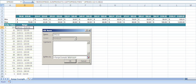
This Excel example will show you how to determine if a cell value is "In Between" a pre-established range. Please see the details below for setup steps and a visual example...

Example Assumptions:

• The spreadsheet has been named: Range Example
• This cell value that you wish to calculate is: A8
• The 'in between' values to check against are placed in cells: B4:L4

Setup Steps:

1. Create your "in between" values somewhere on the spreadsheet (Cells B4:L4 are used in this example)
2. Create a "Named Range". In this example, the Named Range has been called: "SPREAD".
3. In the "Refers to:" field for "SPREAD", enter the following reference: ='Range Example'!$B$4:$L$4
4. Click 'OK' to save the Named Range.
5. Enter the formula below into a cell that's (preferably) adjacent to the cell that you wish to find the range for:

=INDEX(SPREAD,-SUMPRODUCT(-(-(LEFT(SPREAD,FIND(" ",SPREAD)-1))>=(-A8))))

The formula above uses the "SPREAD" Named Range, which you defined earlier, to determine if the referenced cell is 'in between' the pre-established range.

For a visual representation of how to set this up, please see the screen shot below...

Dynamic Range Assignment

Dynamic Referencing for Excel Pivot Table(s) and / or Graph(s)

BC, this one's for you... :-)

Situation: You have an Excel solution that auto generates Graphs and / or Charts based on a specific set of data that changes over time. Instead of manually re-selecting a new Data Source for your Pivot Table(s) and / or Graph(s) each time your Raw Data changes (i.e. appending Q2 data to Q1, etc.), check out the information below for a dynamic solution...

• Excel Sheet Name = "DataTab"
• Column Headers Accross the top beginning with A1
• Subsequent Data lies beneath each Header
• Assuming your data is standardized and consistent over time
• Create a Named Range called "DataRange" and paste in the following formula...

=OFFSET('DataTab'!$A$1,0,0, COUNTA('DataTab'!$A:$A), COUNTA('DataTab'!$1:$1))

• Assign the above Named Range ("DataRange") to your Pivot Table and/or Graph as it's Data Source

• Refresh your Table(s) / Graph(s) - Can be done manually, via Table Settings, or with VBA

When you paste in future data that may be different from your original data, your Graph(s) and / or Chart(s) will now be based on a dynamically growing or shrinking dataset that matches your "evolved" Data Source.

Compare & Consolidate

Excel Value Comparison & Result Consolidation

If This ~ Or That ~ Then This ~ Else This
With raw data in cell(s) A2:xx, place the following formula in cell(s) B2:xx

=IF(OR(ISNUMBER(SEARCH("*Item1*",A2)),(ISNUMBER(SEARCH("*Item2*",A2)))),"Assigned Value",A2)
This formula will search the contents of cell A2 and if it finds anything relating to “Item1” OR “Item2”, it will place the word “Assigned Value” in B2. If it doesn’t find the referring value, it will simply place the existing contents of cell A2 in cell B2.

Excel Nested IF's

A well known limitation to Excel is that you cannot "nest" more than 7 functions. For example, the following formula will fail because the limit is exceeded.

=IF(Sheet1!$A$4=1,11,IF(Sheet1!$A$4=2,22,IF(Sheet1!$A$4=3,33,IF(Sheet1!$A$4=4,44,IF(Sheet1!$A$4=5,55,IF(Sheet1!$A$4=4,44,IF(Sheet1!$A$4=5,55,IF(Sheet1!$A$4=6,66,IF($A$4=7,77,FALSE))))))))

As a general "rule of thumb," if you have a formula with more than 7 nested statements, you should consider using a VBA function instead. However, if you do not want to use VBA, you can get around this limitation by creating a defined name that refers to part of the formula. Since defined formulas are evaluated separately, you can have one or more defined formulas which refer to large formulas, and combine these into a "master" formula.

Suppose we wanted an nested IF formula to test: IF A4 = 1 Then 11 Else If A4 = 2 Then 22 Else If A4 = 3 Then 33 Else If A4 = 4 Then 44...Else If A4 = 55 Then 55 Else "Not Found" and so on.

Of course, as a practical matter, we'd be better off using a VLOOKUP to do this, but this will work for illustration. First, we'd create a named formula called OneToSix, referring to the formula:

=IF(Sheet1!$A$4=1,11,IF(Sheet1!$A$4=2,22,IF(Sheet1!$A$4=3,33,IF(Sheet1!$A$4=4,44,IF(Sheet1!$A$4=5,55,IF(Sheet1!$A$4=4,44,IF(Sheet1!$A$4=5,55,IF(Sheet1!$A$4=6,66,FALSE))))))))

Then create another named formula called SevenToThirteen, referring to the formula:
=IF(Sheet1!$A$4=7,77,IF(Sheet1!$A$4=8,88,IF(Sheet1!$A$4=9,99,IF(Sheet1!$A$4=10,100,IF(Sheet1!$A$4=11,110,IF(Sheet1!$A$4=12,120,IF(Sheet1!$A$4=13,130,"NotFound")))))))

Finally, enter the "master" formula in the worksheet cell: =IF(OneToSix,OneToSix,SevenToThirteen)

It's not pretty, but it can be a work around in a pinch...This "beats" the nested function limitation because no single part of the formula exceeds the limit, even though the "sum" of the components do. You can use this technique whenever you exceed the limit on nested functions.

Excel - Current Quarter Calc

Excel Formula to Calculate the Current Quarter

=IF(LEN(B2) > 0,VLOOKUP(MONTH(B2),{1,"Q1";4,"Q2";7,"Q3";10,"Q4"},2),"") & IF(LEN(B2)>0,IF(OR(MONTH(B2)=1,MONTH(B2)=2)," '" & RIGHT(YEAR(B2),2)," '" & RIGHT(YEAR(B2),2)),"")

Excel - Trim Last 5 Characters

Excel Formula to capture and trim the last 5 characters of an adjacent Field that contains a string value

=RIGHT(C37,LEN(C37)-FIND("*",SUBSTITUTE(C37," ","*",LEN(C37)-LEN(SUBSTITUTE(C37," ","")))))

Excel Progress Indicator

Displaying a Progress Indicator in Excel...

I can't take credit for this code...I found it on the internet at this address: http://j-walk.com/ss/excel/tips/tip34.htm

KUDO's to the original developer, who ever it is...
-----------------------------------
Click HERE to download an example
A common question among Excel developers is, How can I use a custom dialog
box to display the progress of a lengthy macro? This document describes
how to create an attractive progress indicator with minimal effort.
Creating the UserFormFollow the steps below to create the progress indicator UserForm.

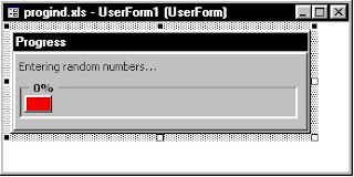
1. Insert a new UserForm and change its Caption to Progress.
2. Add a Frame control and name it FrameProgress.
3. Add a Label control inside of the Frame and name it LabelProgress.
4. Remove the Label's caption, and make its background color red.
5. Add another label (option) to describe what's going on.
6. Adjust the form and controls so they look like this:

Creating the Event-handler subroutines
The trick here involves running a subroutine automatically when the dialog box is displayed. Since the Initialize event occurs before the dialog box is actually show, you must use the Activate event. Insert the following subroutine in the Code window for the UserForm. This subroutine simply calls the Main subroutine (stored in a VBA module) when the UserForm is displayed.
CODE:
-----------------------------------
Private Sub UserForm_activate()
Call Main
End Sub
-----------------------------------
The Main subroutine is listed below. This demo routine simply inserts random numbers into the active worksheet. As it does so, it changes the width of the Label control and displays the percent completed in the Frame's caption. You will, of course, substitute your own subroutine. And you'll need to figure out how to determine the progress complete.
-----------------------------------
CODE Continued:
Sub Main()

' Inserts random numbers on the active worksheet
Dim Counter As Integer
Dim RowMax As Integer, ColMax As Integer
Dim r As Integer, c As Integer
Dim PctDone As Single
If TypeName(ActiveSheet) <> "Worksheet" Then Exit Sub
Cells.Clear
Application.ScreenUpdating = False
Counter = 1
RowMax = 100
ColMax = 25
For r = 1 To RowMax
For c = 1 To ColMax
Cells(r, c) = Int(Rnd * 1000)
Counter = Counter + 1
Next c
PctDone = Counter / (RowMax * ColMax)
With UserForm1
.FrameProgress.Caption = Format(PctDone, "0%")
.LabelProgress.Width = PctDone * (.FrameProgress.Width - 10)
End With
' The DoEvents statement is responsible for the form updating
DoEvents
Next r
Unload UserForm1
End Sub
-----------------------------------
Creating the start-up subroutine
All that's missing is a subroutine to display the dialog box. Enter the following subroutine in a VBA module.
-----------------------------------
CODE Continued:
Sub ShowDialog()
UserForm1.LabelProgress.Width = 0
UserForm1.Show
End Sub
-----------------------------------
How it works
When you execute the ShowDialog subroutine, the Label object's width is set to 0. Then the Show method of the UserForm1 object displays the dialog box. When the dialog box is displayed, its Activate event is triggered, which executes the Main subroutine. The Main subroutine
periodically updates the width of the Label. Notice the DoEvents statement. Without this statement, changes to the Label are not visible. Before the subroutine ends, the last statement unloads the UserForm object.
Caveat
This is definitely a slick technique, but you should be aware that it may slow down your macro a bit due to the extra overhead of updating the progress indicator. In many cases, however, it is not even noticeable.

Excel Formula comparison (If~Then~AND~Else)

=IF(AND(E14="",D14<>""),"No Personal Miles","")

Excel Formula to count word instances in a column based on 2 different criteria

=SUMPRODUCT(('Raw Data Tab'!$K$2:$K$15=$A3)*('Raw Data Tab'!$L$2:$L$15=I$1))

#N/A Trap and VLookup Combo

Excel Formula to trap for #N/A and perform another VLookup using a modified KEY Value


=IF(ISNA(VLOOKUP(D2,'Goal and Activity
Data'!$D$2:$Y$795,3,FALSE)),VLOOKUP(LEFT(D2,LEN(D2)-2),'Goal and Activity
Data'!$D$2:$Y$795,3,FALSE),(VLOOKUP(D2,'Goal and Activity
Data'!$D$2:$Y$795,3,FALSE)))